Software

One of my research interests is in developing algorithms to answer the most pressing questions in astrophysics. These include searching for novel signals from technologically-advanced extraterrestrial life; finding Fast Radio Bursts; studying the observational properties of pulsars and megnetars. Following are a few of the software tools I have developed over the years.

Mobirise
SPANDAK 

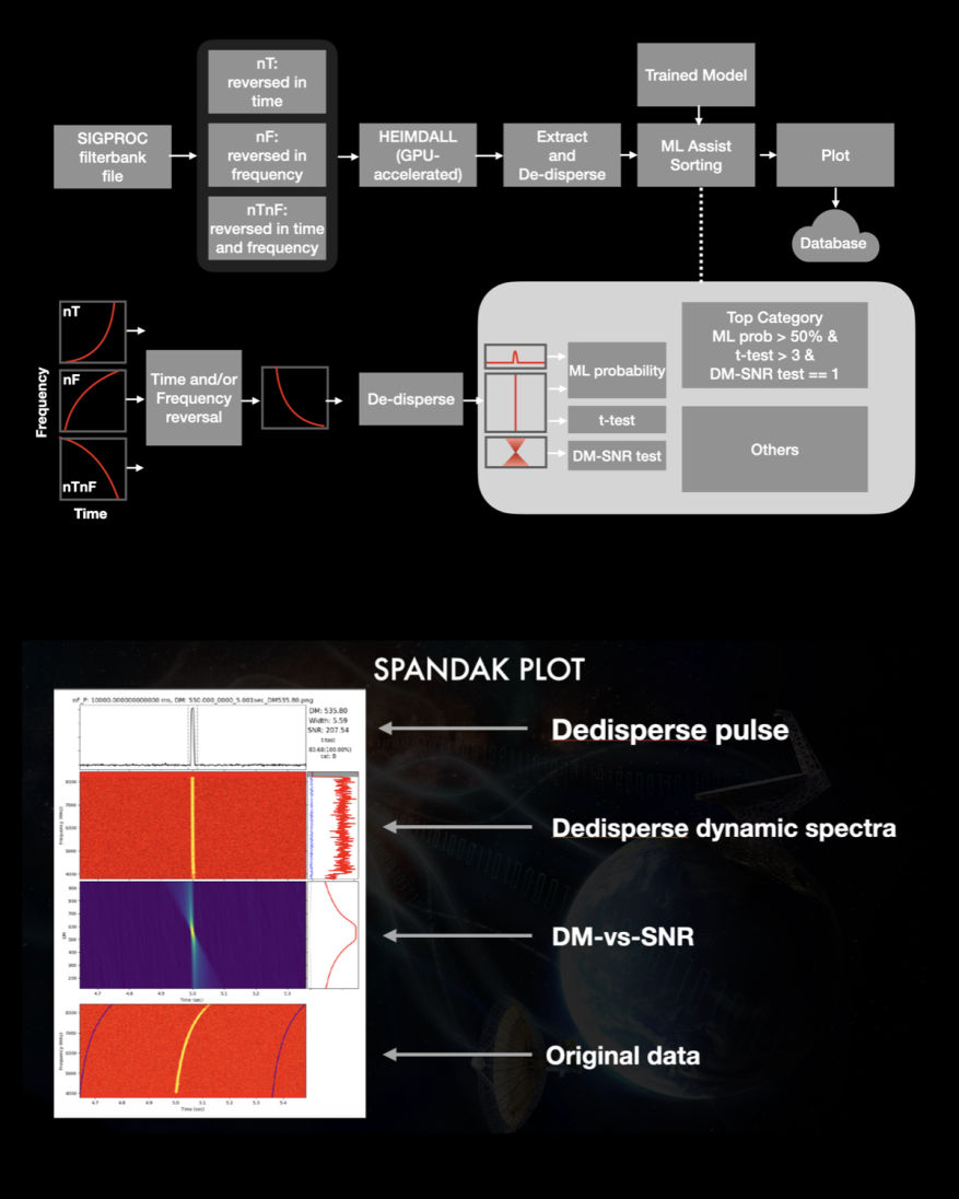
SPANDAK (in Hindi: pulsating objects) is a python wrapper built around a GPU-accelerated tool — named HEIMDALL (Barsdell et al. 2012) — as the main kernel to search for dispersed signals of natural and artificial origin. It uses a SIGPROC-based filterbank file to search for dispersed pulses from a user-supplied range of DMs and pulse widths. The pipeline accumulates all transient candidates reported with HEIMDALL and cross-references various candidate parameters (proximity of arrival times, DMs, S/Ns, widths, etc.). It removed candidates that appear across a large range of DMs within a short interval, allowing us to remove a significant number of false positives due to RFI. A short list of selected candidates gets extracted from each corresponding filterbank file for further validation. SPADNAK time-scrunches the extracted data such that the detected pulse would fit within two to four-time bins and frequency scrunched 16-512 frequency bins. For candidate validation, the pipeline produces dedispersed dynamic spectra, where an ideal broadband transient pulse should show up across all observed frequencies. The pipeline then selects an on-pulse window based on the width and arrival time reported from HEIMDALL and extracts on-pulse and off-pulse spectra. Pipeline compares the on-pulse and off-pulse spectral energy distribution using a t-test. For a true broadband pulse, the t-test shows a significant difference between these spectra. Moreover, a true broadband dispersed signal shows both a peak at the correct DM and a gradual decline in the S/N around nearby DMs. SPANDAK then produces plots for each of the candidates for visual inspection by the user. 

Mobirise
Clustering in time-series using Pair Correlation Function (PCF) 

The Pair Correlation Function (PCF) is a probability density function (also known as the radial distribution function or pair separation function) for the clustering of certain objects or events in space and/or time coordinates (Pimbley & Lu 1985) and is useful for measuring the degree of packing. This code uses one-dimensional PCF, which identifies the clustering of events in the time series data. The PCF for a series M pulses with N burst pulses can be derived as follows. The pulse index of these burst pulses are pi or pj = p1, p2, ..., pN. Then, PCF is defined as; 
PCF(p) = G·∑∑⟨δ(p − |pj−pi|)⟩.
Where G is a scaling parameter and δ is the Kronecker delta function. A normalized binning of PCF, provides the probability of occurrence of certain separations between burst pulses. If any time-series exhibits bunching of events and periodic occurrence of these bunches, the PCF shows prominent peaks around repeatedly occurring separations and their harmonics. A simple way to detect such periodicities is to obtain the Fourier spectra of the PCF. 

Mobirise
MACHINE LEARNING ASSISTED SPANDAK 


WHAT: To prioritize visual inspection by user, we build a convolution neural
network classifier. This has helped us reject 97% of false positives. We achieved this by training the ML classifier to classify dedispersed dynamic spectra and frequency-averaged pulses. Modern supervised learning methods require large amounts of training data, so we created a synthetic data set of a wide variety of mock broadband signals embedded in the background of real telescope noise and spurious RFI. A total of around 200,000 data points were simulated, in which 100,000 of these synthetic data contained mock broadband signals embedded in real telescope backgrounds, and the remaining 100,000 contained empty backgrounds.

HOW: For every example, the model takes two inputs, a 2D dynamic spectrum, and its corresponding 1D frequency-averaged time series. These inputs are fed into two separate branches of the network —what we call the spectrogram branch and the time series branch—which extract features from the inputs and are eventually concatenated together to produce one softmax prediction. We found that architecture with two convolutional layers worked best for our application, retaining the ability to recognize signals without being unnecessarily complex. A 3 × 3 kernel with a stride length of 1 ensures that the convolution operation does not “skip over” broken broadband signals. In the time series branch, the number of filters in a convolutional layer is roughly half the number of filters in the parallel convolutional layer in the spectrogram branch to prevent overfitting, since detecting whether a peak is present in a 1D signal is not a hugely complex task. Each convolutional layer is followed by a BatchNormalization layer and a ReLU activation. We use MaxPooling layers at the end of every convolutional block in the spectrogram branch to reduce the dimensionality but found that MaxPooling layers within the time series branch led to losing the peaks in the 1D signal and thereby decided to remove them. After all convolutional blocks for both branches, we use global max pooling to transform all convolutional feature maps into a 1D tensor for each example. Subsequently, the two branches of the network are fused by concatenating the outputs of the GlobalMax- Pooling layers, after which they are fed into two fully connected layers before the prediction layer. We also use Dropout layers between the fully connected layers, which are a simple method of reducing overfitting.

TRAINING: We implement our classifier in Keras 2.0.8 and TensorFlow 1.4.1, compiling the model with a binary cross-entropy loss and the Adam optimizer Because we value recall over precision, we weight the positive class 10 times as much as the negative class, thereby penalizing the network more for missing signals than for false positives. We employ several Keras callbacks to supplement model training: ModelCheckpoint, ReduceLROnPlateau, and EarlyStopping. With a batch size of 32, we trained our models using a single Nvidia Titan XP GPU. With the validation set throughout training 134 epochs, our model converged with a validation recall of 0.9897.

Mobirise
Barycentric correction of filterbank files 

Narrowband radio signals with extremely limited spectral occupancy (<<1 Hz) are prime candidates for potential beacons from Extraterrestrial Intelligent (ETI) civilizations. These signals drift in frequency as line-of-sight acceleration changes due to Earth's rotation. Given a user-supplied SIGPROC filterbank file, this code corrects for the Earth's rotation towards the source and moves topocentric observing frequencies to barycentric frequencies. While observing the same target from two widely separated telescopes, this software allows the comparison of narrowband signals at both stations in the barycentric frame of reference; hence providing the best possible way to discriminate terrestrial interference from a truly sky-localised signal. The top two panels in the figure show narrowband signals detected at Sweden and Ireland LOFAR stations in the Topocentric frame. The bottom two panels show narrowband signals at these stations in the Barycentric frame showing a significant difference in the drift rates due to the signal's terrestrial origin.

Set up a site with Mobirise